Self-supervised Learning: What is? and A case study (SimCLR)
Introduction
In traditional supervised learning, a labeled dataset is used to train a machine learning model to make predictions on new, unseen data. However, in self-supervised learning, the model learns from unlabeled data and creates its own labels or annotations through various techniques. These labels or annotations are then used to train the model in a supervised manner. Self-supervised learning allows for more efficient use of large amounts of unlabeled data and can be used in situations where labeled data is scarce or expensive to obtain.
Why self-supervised learning is important in the context of computer vision?
Self-supervised learning is important in the context of computer vision because it allows for the efficient use of large amounts of unlabeled data to train deep learning models. With the explosion of digital data and the availability of powerful computing resources, there is an abundance of unlabeled data available that can be used to train computer vision models. However, traditional supervised learning methods rely on labeled data, which can be scarce and expensive to obtain. By contrast, self-supervised learning allows models to learn from unlabeled data and create their own labels or annotations, making it possible to train more accurate and robust models with much less labeled data. This is especially important in computer vision applications where the cost and effort of labeling data can be prohibitively high, such as in medical imaging, satellite imagery analysis, and autonomous driving.
What is self-supervised learning?
Self-supervised learning is a type of machine learning that allows a model to learn from unlabeled data by creating its own supervisory signal or annotation. This is achieved by defining a surrogate or proxy task that is easy to solve using the unlabeled data, but which requires the model to capture important patterns or relationships in the data. The model then uses the output of the surrogate task as its supervisory signal or annotation to train itself in a supervised manner. Examples of self-supervised learning include:
- Contrastive learning: This technique trains a model to learn embeddings of input data such that semantically similar examples are mapped to nearby points in the embedding space, while dissimilar examples are mapped to distant points. The model is trained using pairs of augmented examples that are either from the same or different classes.
- Predictive coding: This technique trains a model to predict future observations or features of the input data. The model is trained using a sequence of input data where each time step is encoded by the model and then decoded to reconstruct the original input. The reconstruction error is then used to train the model.
- Generative models: This technique trains a model to generate new samples that are similar to the input data. The model is trained using the input data to learn a probability distribution over the data, and then generates new samples by sampling from this distribution.
Self-supervised learning differs from other types of unsupervised learning in that it involves creating a supervisory signal or annotation from the input data itself, rather than relying on external labels or annotations. This makes it more efficient and scalable than traditional supervised learning, and allows for the use of much larger amounts of unlabeled data. In contrast, other types of unsupervised learning, such as clustering or dimensionality reduction, do not involve creating a supervisory signal or annotation, and instead focus on finding patterns or structure in the input data.
A case study: SimCLR
This tutorial explores self-supervised contrastive learning, a type of unsupervised learning where input data is given without accompanying labels. Self-supervised learning methods aim to learn from the data alone, making it useful for quickly fine-tuning models for specific classification tasks. The benefit of self-supervised learning is the ability to obtain large datasets without manual labeling. Contrastive learning is a subfield of self-supervised learning that trains a model to cluster an image and its slightly augmented version in latent space while maximizing the distance to other images. SimCLR is a recent and straightforward method for contrastive learning. The overral framework has been depicted in Fig.1.
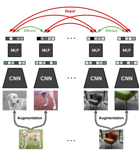 Fig.1 - SimCLR framework.
The objective is to train a model on a dataset of unlabeled images to adapt quickly to any image recognition task. During training, a batch of images is sampled, and two versions of each image are created through data augmentation techniques. A CNN like ResNet is used to obtain a 1D feature vector on which a small MLP is applied. The output features of the augmented images are trained to be close, while all other images in the batch should be as different as possible. This trains the model to recognize the unchanged content of the image under augmentations, such as objects.
Data Augmentation
The first step is to define the data augmentation techniques we will use to create different views of the same image. Common data augmentation techniques include random cropping, random flipping, color jittering, and Gaussian blurring.
import torchvision.transforms as transforms


# Define data augmentation transformations
train_transform = transforms.Compose([
    transforms.RandomResizedCrop(size=224, scale=(0.2, 1.0)),
    transforms.RandomHorizontalFlip(),
    transforms.ColorJitter(brightness=0.4, contrast=0.4, saturation=0.4, hue=0.1),
    transforms.RandomApply([transforms.GaussianBlur(kernel_size=3)], p=0.5),
    transforms.ToTensor(),
    transforms.Normalize(mean=[0.485, 0.456, 0.406], std=[0.229, 0.224, 0.225])
])
import torchvision.models as models
# Load a pre-trained ResNet-18 model
encoder = models.resnet18(pretrained=True)
# Replace the last fully connected layer with an identity function
encoder.fc = nn.Identity()Projection Head
The projection head is used to project the feature vectors into a lower-dimensional space. We can use a simple MLP with two hidden layers for the projection head.
# Define a simple MLP projection head
class MLP(nn.Module):
    def __init__(self, input_dim=512, hidden_dim=256, output_dim=128):
        super(MLP, self).__init__()
        self.layer1 = nn.Linear(input_dim, hidden_dim)
        self.layer2 = nn.Linear(hidden_dim, output_dim)

    def forward(self, x):
        x = F.relu(self.layer1(x))
        x = self.layer2(x)
        return x

projection_head = MLP()
Contrastive Loss
The contrastive loss is used to maximize the agreement between different views of the same image, and minimize the agreement between different images. We can use a temperature-scaled softmax function to compute the contrastive loss.
# Define the contrastive loss function
class ContrastiveLoss(nn.Module):
    def __init__(self, temperature=0.5):
        super(ContrastiveLoss, self).__init__()
        self.temperature = temperature

    def forward(self, z_i, z_j):
        batch_size = z_i.shape[0]
        z = torch.cat([z_i, z_j], dim=0)
        sim_matrix = torch.exp(torch.mm(z, z.t().contiguous()) / self.temperature)
        mask = torch.eye(batch_size, dtype=torch.bool)
        loss = (sim_matrix - torch.diag(sim_matrix.diagonal())).sum() / (2 * batch_size - 2)
        return loss
Training Loop
To train the SimCLR model, we need to sample two views of each image, encode them using the pre-trained encoder network, project them using the projection head, and compute the contrastive loss. We can train the model using stochastic gradient descent (SGD) with a learning rate schedule and a momentum term.
import torch.optim as optim

# Define the optimizer and learning rate schedule
optimizer = optim.SGD(list(encoder.parameters()) + list(projection_head.parameters()), lr=0.3, momentum=0.9, weight_decay=1e-4)
lr_scheduler = optim.lr_scheduler.CosineAnnealingLR(optimizer, T_max=10)

# Train the model for a number of epochs
for epoch in range(num_epochs):
    for batch_idx, (images, _) in enumerate(train_loader):
        # Sample two views of each image
        images = torch.cat([images, images.flip(3)], dim=0)
        # Encode the images using the pre-trained encoder
        features = encoder(images)
        # Project the features using the MLP projection head
        projections = projection_head(features)
        # Split the projections into two parts
        z_i, z_j = torch.chunk(projections, 2, dim=0)
        # Compute the contrastive loss
        loss = contrastive_loss(z_i, z_j)
        # Update the parameters using stochastic gradient descent
        optimizer.zero_grad()
        loss.backward()
        optimizer.step()
        # Update the learning rate
        lr_scheduler.step()
Evalutation
TO evaluate the performance of the SimCLR model on a held-out test set:
# Evaluate the performance of the SimCLR model on a held-out test set
with torch.no_grad():
    # Set the model to evaluation mode
    encoder.eval()
    projection_head.eval()

    # Create empty lists to store the representations and labels
    representations = []
    labels = []

    # Loop over the test set and compute the representations and labels
    for images, target in test_loader:
        # Encode the images using the pre-trained encoder
        features = encoder(images)
        # Project the features using the MLP projection head
        projections = projection_head(features)
        # Add the projections and labels to the lists
        representations.append(projections)
        labels.append(target)

    # Concatenate the representations and labels into tensors
    representations = torch.cat(representations, dim=0)
    labels = torch.cat(labels, dim=0)

    # Compute the cosine similarity matrix between the representations
    sim_matrix = F.normalize(torch.mm(representations, representations.t()), dim=1)

    # Compute the top-1 and top-5 classification accuracies
    top1_acc = 0.0
    top5_acc = 0.0
    for i in range(len(test_dataset)):
        # Get the row of the similarity matrix corresponding to the current image
        sim_row = sim_matrix[i]
        # Get the indices of the images with the highest cosine similarity to the current image
        top5_idx = torch.argsort(sim_row, descending=True)[:5]
        top1_idx = top5_idx[0]
        # Check if the true label is among the top-5 predicted labels
        if labels[i] in labels[top5_idx]:
            top5_acc += 1.0
        # Check if the true label is the top-1 predicted label
        if labels[i] == labels[top1_idx]:
            top1_acc += 1.0

    # Compute the final accuracies
    top1_acc /= len(test_dataset)
    top5_acc /= len(test_dataset)

print(f"Top-1 Accuracy: {top1_acc:.4f}")
print(f"Top-5 Accuracy: {top5_acc:.4f}")
Conclusion
This tutorial introduced self-supervised contrastive learning and demonstrated its implementation using SimCLR as an example method. Recent research, including Ting Chen et al., has shown that larger datasets like ImageNet exhibit similar trends. In addition to the discussed hyperparameters, the model size also plays a crucial role in contrastive learning. If abundant unlabeled data is available, larger models can achieve stronger results and come close to their supervised counterparts. Additionally, combining contrastive and supervised learning approaches, as shown in Khosla et al., can result in performance gains beyond supervision.
It’s worth noting that contrastive learning is not the only self-supervised approach that has gained attention in recent years. Other methods, such as distillation-based methods like BYOL and redundancy reduction techniques like Barlow Twins, have also shown promising results. There is still a lot to explore in the self-supervised domain, and we can expect further impressive advances in the near future.
References
- He, K., Fan, H., Wu, Y., Xie, S., & Girshick, R. (2020). Momentum contrast for unsupervised visual representation learning. In Proceedings of the IEEE/CVF Conference on Computer Vision and Pattern Recognition (pp. 9729-9738).
- Lotter, W., Kreiman, G., & Cox, D. (2017). Deep predictive coding networks for video prediction and unsupervised learning. In International Conference on Learning Representations.
- Goodfellow, I., Pouget-Abadie, J., Mirza, M., Xu, B., Warde-Farley, D., Ozair, S., … & Bengio, Y. (2014). Generative adversarial nets. In Advances in neural information processing systems (pp. 2672-2680).
- Chen, T., Kornblith, S., Norouzi, M., & Hinton, G. (2020). A simple framework for contrastive learning of visual representations. In International Conference on Machine Learning (pp. 1597-1607).
- Grill, J. B., Strub, F., Altché, F., Tallec, C., Richemond, P. H., Buchatskaya, E., … & Piot, B. (2020). Bootstrap your own latent: A new approach to self-supervised learning. arXiv preprint arXiv:2006.07733.
- Chen, Y., Kalantidis, Y., Li, J., Yan, S., & Feng, J. (2020). CCL: Contrastive learning for weakly supervised object detection. In Proceedings of the IEEE/CVF Conference on Computer Vision and Pattern Recognition (pp. 11449-11458).